Compressed Kernel Density Estimation (cKDE)

Kernel density estimation is a non-parameteric method to estimate a (unknown) probability density from a set of data samples. In essence, each data sample is replaced by a kernel function with a bandwidth parameter that determines the smoothness of the density (see the math section below).

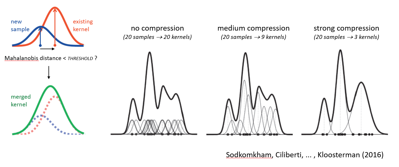
If there are many data samples, then computing the kernel density estimate can be quite computationally expensive. In our effort to develop a method for real-time neural decoding, we used an approach that made direct use of spike waveform features without an intermediate spike-sorting step (Kloosterman et al., 2014). However, this approach was relatively slow because we relied on evaluation of kernel densities. To speed up the computation, we made use of redundancy in the data and expressed the kernel density with fewer kernels than data samples by merging nearby samples into “super-samples” (Sodkomkam et al., 2016). The level of compression (and hence the trade-off with accuracy) is controlled by a threshold on the mahalanobis distance between a new data sample and the nearest existing kernel in the density. The kernel merging approach is illustrated in the figure below.

Math

Kernel density estimation

For a d-dimensional space in which a point’s location is given by the d-vector of coordinates \(\boldsymbol{x}=(x_1, x_2, \dots, x_d)\), a kernel density \(f(\boldsymbol{x})\) is expressed as the weighted sum of \(n\) kernels centered on locations \(\boldsymbol{M} = \left[\boldsymbol{\mu}_1, \dots, \boldsymbol{\mu}_n\right]\), with scales (bandwidths) \(\boldsymbol{H} = \left[\boldsymbol{h}_1, \dots, \boldsymbol{h}_n\right]\) and weights \(\boldsymbol{w}=\left[w_1, \dots, w_n\right]\):

\(f(\boldsymbol{x})=\sum_{i=1}^{n}{w_i K\left(\boldsymbol{x}; \boldsymbol{\mu}_i, \boldsymbol{h_i}\right)}\)

Here, \(\boldsymbol{\mu}_i\) and \(\boldsymbol{h}_i\) are d-vectors of coordinates and bandwidths for each dimension of kernel i. Further, \(\sum_{i=1}^{n} w_i = 1\) and the kernel \(K\) is a probability distribution, i.e. positive for all \(\boldsymbol{x}\) and \(\int K(\boldsymbol{x})d\boldsymbol{x}=1\).

Generally, the kernel centers coincide with the data samples \(\boldsymbol{x}_i\), the kernel bandwidth is fixed for all kernels and the weights all equal \(\frac{1}{n}\).

There are many kernel functions to choose from (e.g., see here). Below a few kernels that we have implemented are listed.

Gaussian kernel

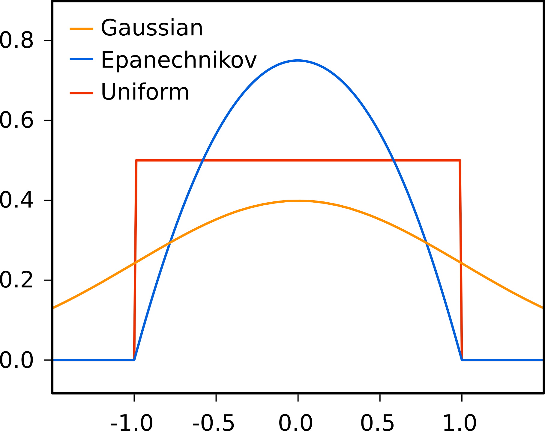
The most common kernel used in kernel density estimation is the gaussian kernel. The multivariate radially symmetric gaussian kernel in d dimensions is given by:

\(K_g(\boldsymbol{x}; \boldsymbol{\mu}, \boldsymbol{h})=\frac{R_d}{(2\pi)^{\frac{d}{2}} \times h_1 \cdots h_d}e^{-\frac{1}{2}\left\Vert\frac{\boldsymbol{x}-\boldsymbol{\mu}}{\boldsymbol{h}}\right\Vert^2}\)

To speed up computation, it can be benificial to only consider the gaussian kernel on a finite support \(\left[-\sigma_{cut},\sigma_{cut}\right]\) for each dimension (here, \(\sigma_{cut}\) is the cut-off in standard deviations). In the equation above, \(R_d\) rescales the gaussian to account for the reduced support region:

\(R_d=\left(1-erfc\left(\frac{\sigma_{cut}}{\sqrt{2}}\right)\right)^{-d}\)

Epanechnikov kernel

The multivariate radially symmetric epanechnikov (or parabolic) kernel in d dimensions is given by:

\(K_e(\boldsymbol{x}; \boldsymbol{\mu}, \boldsymbol{h})=\frac{d+2}{2V_d \times h^*_1 \cdots h^*_d }\left(1-\left\Vert \frac{\boldsymbol{x}-\boldsymbol{\mu}}{\boldsymbol{h^*}}\right\Vert^2\right)\)

Here, \(V_d\) is the volume of the unit hypersphere: \(V_d = \frac{\pi^{\frac{d}{2}}}{\Gamma\left(\frac{d}{2}+1\right)}\)

The epanechnikov kernel has finite support, i.e. \(\left\Vert\frac{\boldsymbol{x}-\boldsymbol{\mu}}{\boldsymbol{h^*}}\right\Vert \leq 1\), and is zero outside that support.

In the above formulation, the bandwidth \(\boldsymbol{h}\) is equivalent to the standard deviation of the gaussian kernel for ease of comparison (this means that for a bandwidth value of 1, the variance of the kernel equals 1). To accomplish this, the bandwidth is scaled by a factor \(\sqrt{5}\), i.e. \(h^* = h \sqrt{5}\).

Uniform kernel

The multivariate radially symmetric uniform (or box) kernel in d dimensions is given by:

\(K_u(\boldsymbol{x}; \boldsymbol{\mu}, \boldsymbol{h})=\frac{1}{V_d \times h^*_1 \cdots h^*_d} \mathbb{1}\left\{ \left\Vert \frac{\boldsymbol{x} - \boldsymbol{\mu}}{\boldsymbol{h}^*}\right\Vert\leq 1 \right\}\)

Again, \(V_d\) is the volume of the unit hypersphere. \(\mathbb{1}\) is the indicator function that equals 1 when the condition in curly brackets is met, and 0 otherwise.

In the above formulation, the bandwidth \(\boldsymbol{h}\) is equivalent to the standard deviation of the gaussian kernel for ease of comparison (this means that for a bandwidth value of 1, the variance of the kernel equals 1). To accomplish this, the bandwidth is scaled by a factor \(\sqrt{3}\), i.e. \(h^* = h \sqrt{3}\).

Von Mises kernel for circular variables

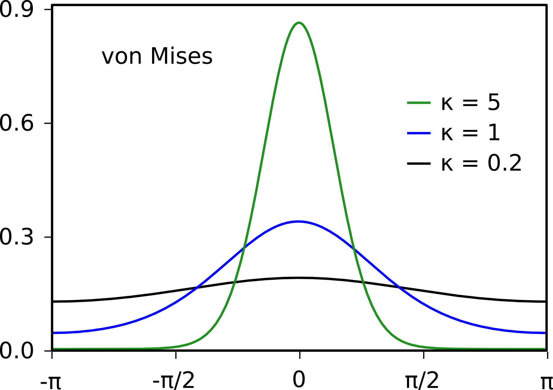
For circular variables such angles or directions, the von Mises kernel is often used. The univariate von Mises kernel for circular variables is given by:

\(K_{vm}(x; \mu, \kappa)=\frac{e^{\kappa \cos(x-\mu)}}{2\pi I_0(\kappa)}\)

Here we use the standard symbol \(\kappa\) for the bandwidth (or concentration) of the von Mises kernel. We only have implemented the univariate von Mises kernel. A multivariate product kernel can be obtained by multiplication of univariate kernels (see below).

For large values of the bandwidth \(\kappa\), the von Mises kernel can be approximated by a gaussian kernel with bandwidth \(\sqrt{\frac{1}{\kappa}}\).

Kronecker delta kernel for categorical variables

For a categorical variable with \(c\) categories, we can use a kronecker delta kernel with integer location \(\mu \in \{0,1,\dots,c\}\). This kernel avoids any smoothing over the categories. Note that the kronkecker delta kernel does not have a bandwidth.

\(K_{\delta}(x; \mu)= \begin{cases} 0 & x \neq \mu \\ 1 & x = \mu \end{cases}\)

Multiplicative (product) kernel

Multiple kernels can be combined into a single multivariate product kernel through multiplication:

\(K(\boldsymbol{x}; \boldsymbol{\mu}, \boldsymbol{h})=K(x_1; \mu_1, h_1) \cdots K(x_p; \mu_p, h_p)\)

Merging of kernels

Gaussian, epanechnikov and uniform kernels

Given two kernels centered at \(\mu_A\) and \(\mu_B\) with bandwidths \(\sigma_A\) and \(\sigma_B\) and weights \(p_A\) and \(p_B\), we can construct another kernel with center \(\mu\), bandwidth \(\sigma\) and new weight \(p=p_A+p_B\) that best approximates the sum of the kernels A and B:

\(\mu = \frac{p_A \mu_A + p_B \mu_B}{p_A + p_B}\)

\(\sigma^2 = p_A \left(\sigma_A^2 + \mu_A^2 \right) + p_B \left(\sigma_B^2 + \mu_B^2 \right) - \mu^2\)

Von Mises kernel

The general merging approach for the von Mises kernel is the same as for the gaussian kernel, but with adaptation to circular variable space:

\(\mu = G\left(\mu_A + \frac{p_A}{p_A + p_B} F(\mu_B - \mu_A)\right)\)

\(\frac{1}{\kappa} = \frac{p_A}{\kappa_A} + \frac{p_B}{\kappa_B} - p_A p_B\left(\pi-|\pi-|\mu_A-\mu_B||\right)^2\)

Here,

\(F(x) = \begin{cases} x+2\pi & x \leq -\pi \\ x-2\pi & x \gt \pi \\ x & otherwise \end{cases}\)

and

\(G(x) = \begin{cases} x+2\pi & x \lt 0 \\ x-2\pi & x \gt 2\pi \\ x & otherwise \end{cases}\)

Other kernels

Two kronecker delta kernels are only merged if their locations are the same, i.e. \(\mu_A=\mu_B\). In that case, the weight of the kernel is updated: \(p=p_A+p_B\).

For a multivariate kernel, the merging is performed separately for each dimension.

Python API cKDE

The compressed kernel density estimation method is available as part of the py-compressed-kde package (documentation). It is implemented in C++ and has a Python binding (created with pybind11).

In Python, after installation, the code is available as part of the compressed_ke module. Below, we first present the the main components of the library and then give a general workflow.

Spaces and Grids

To compute the compressed kernel density, one first has to describe the space of the variables (i.e., euclidean, circular, categorical, encoded or any combination of these spaces) and one has to specify a grid of points at which the density needs to be evaluated.

Euclidean Space

The euclidean space is used for most continuous variables. In d-dimensional euclidean space, the distance between two d-vector data samples is computed as \(\Vert\boldsymbol{x}-\boldsymbol{y}\Vert\). Three kernels are available: gaussian, epanechnikov and uniform (box) kernels.

To construct a euclidean space, you provide labels for all dimensions, a kernel object (GaussianKernel, EpanechnikovKernel or BoxKernel) and kernel bandwidths for all dimensions.

space = EuclideanSpace(
    [label, label, ...],      # list of labels for all dimensions
    kernel=GaussianKernel(),  # desired kernel
    bandwidth=[1, 1, ...]     # list of bandwidths for all dimensions
)

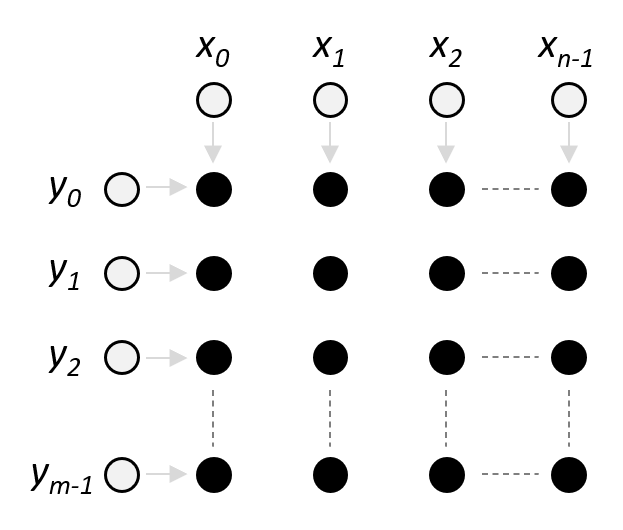
Evaluation of a euclidean space is performed on a regular rectangular grid. To create this grid, you use the grid method of the space object and provide a list of vectors that specify the grid coordinates for each dimension (see image on the right). Optionally, you can provide a boolean valid array with the same number of point as the grid to indicate which grid points should be evaluated (by default evaluation is performed for all grid points). This is useful when the region of interest is not rectangular.

grid = space.grid(
    [x, y, ...],  # list of coordinate vectors for all dimensions
    valid=[],     # boolean array to indicate grid points to be evaluated
    selection=[]  # boolean vector to indicate subset of dimensions for grid
)

Circular Space

The circular space is used for angle or direction variables that are measured in radians or degrees. Only univariate (1D) circular spaces are supported, but multiple circular spaces can be combined in a Multi Space. This distance between two samples in a circular space is computed as \(\pi-|\pi-(x-y)|\). Circular spaces use the von Mises kernel, which for large enough concentration paramater \(\kappa\) can be approximated by a gaussian kernel.

To construct a circular space, provide a label and the default concentration \(\kappa\) for the von Mises kernel.

space = CircularSpace(
    label,    # the name of the space
    kappa=5,  # concentration for von Mises kernel
    mu=0      # center for von Mises kernel
)

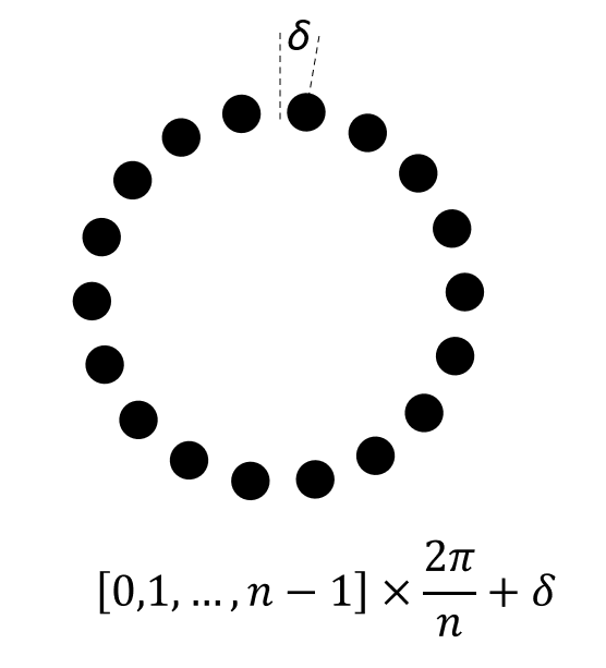
The evaluation grid of a circular space is a regularly-spaced vector of points around the circle (see image on the right). The construct the grid, use the grid method of the space object and provide the number of grid points, and optionally a rotational offset:

grid = space.grid(
    n=24,     # number of grid points around the circle
    offset=0  # rotational offset
)

Categorical Space

The categorical space is used for discrete stimuli, for example running direction on a linear track (outbound/inbound) or discrete visual stimuli. The distance between categorical data samples \(x\) and \(y\) is zero only when \(x=y\) and infinite when \(x \neq y\). The associated kernel is the Kronecker delta kernel.

You can construct a categorical space as follows:

space = CategoricalSpace(
    label,      # the name of the space
    categories, # a list of category labels
    default=0   # index of the default category for new kernels
)

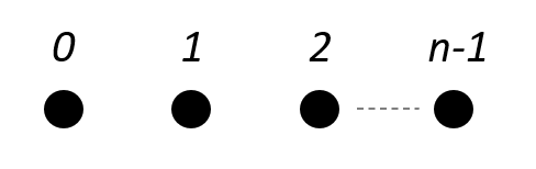
The evaluation grid for a categorical space is the zero-based list of category indices, as visualized on the right. To construct this grid, use the grid method of the space object:

grid = space.grid()

Encoded Space

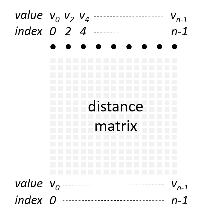
An encoded space can be used for cases that are not covered by the euclidean space, circular space or categorical space. An example from our data is the position on a multi-arm track woth choice points. We can “linearize” the position on the track, but this will result in discontinuities and thus a euclidean space cannot be used. An encoded space is defined by a custom function that computes the (squared) distance between any two data samples in the space. In practice, the space is discretized at \(n\) fixed points \(\boldsymbol{v}=[v_0,v_1,\dots,v_{n-1}]\) and distances are pre-computed for all pairs of points (see distance matrix in image on the right). Each discretized point can either be referred to by their index \(i \in \{0,1,\dots,n-1\}\) or their value \(v_i\). The encoded space has no notion of dimensionality beyond the supplied distance matrix. To compute the kernel density, the encoded space uses a gaussian kernel to convert bandwidth-normalized distance to probability.

There are two ways to construct an encoded space, depending on whether one provides the value vector \(\boldsymbol{v}\) or not. When a label, distance matrix and desired kernel bandwidth, but no value vector is provided, then points in the space (e.g. the grid) are referred to by their indices in the distance matrix:

space = EncodedSpace(
    label,      # name of the space
    distances,  # (n,n) array of squared distances
    bandwidth=1 # kernel bandwidth
)

Alternatively, a value vector can be provided and points in the space (e.g. the grid) are referred to by their associated value. For the multi-arm track example, values could be the linearized position on the track.

space = EncodedSpace(
    label,      # name of the space
    values,     # vector of values associated to discretized points
    distances,  # (n,n) array of squared distances
    bandwidth=1 # kernel bandwidth
)

To construct a grid for evaluation, call the grid method of the space object. The only argument is delta, which specifies the subsampling interval of the discretized points to select the points for evaluation (delta=2 means that one in every two points is selected for the grid). In this way, the internal computations (locations of merged kernels) are performed at a fine scale and evaluation is performed at a coarser scale. The grid method takes care internally of specifying the grid in indices or values.

grid = EncodedSpace.grid(
    delta=1  # subsampling interval
)

Multi Space

A MultiSpace object is a container for any combination of Euclidean, categorical, circular and encoded spaces. The computation of distance between two points in the space is delegated to the child spaces. The associated kernel is a multiplicative kernel of the child space kernels.

To construct a MultiSpace object, pass in a list of child space objects:

space = MultiSpace([space, space, ...])

And to construct a grid, first construct grids for each of the child spaces and then pass these as a list to the space grid method:

grid = space.grid(
    [grid, grid, ...]
)

Mixture

A Mixture object is a container for (potentially merged) data samples and their associated kernels. New data samples can be added (add method) without merging with existing kernels, or merged (merge method). Evaluation of the density on a pre-defined grid of points is done with the evaluate method.

Workflow for compressed kernel density estimation

Step 1: Build model

First, construct a space object that is appropriate for your variables of interest.

space_xy = EuclideanSpace(["x", "y"], bandwidth=[5.0, 5.0])

# other examples
# space_angle = CircularSpace(“angle”, kappa=5.0)
# space = CategoricalSpace(“direction”, [“inbound”, “outbound”])
# space = EncodedSpace(“position”, distance, bandwidth=5.0)
# space = MultiSpace([space_xy, space_angle])

Next, construct a mixture object that will hold the data samples (possibly merged into super-samples) for later evaluation of the density. Choose the compression to balance accuracy and compute time. Note that the compression was developed for online applications for which low latency computations are required. A compression value of 1.0 or 1.5 provides significant speed-ups without much degradation of the estimate. For offline applications, you could choose to lower the compression. Note that the density estimation is not optimized for zero compression and other libraries are likely faster (but may not support all types of spaces).

mix = kde.Mixture(space_xy, compression=1.0)

Add data samples to the mixture. By using the merge method, data samples that are close to existing samples in the mixture are merged into a super-sample. If neighboring data samples are correlated, it is beneficial to merge the samples in a random order to improve the overall kernel density estimate. By default, data samples are randomized before merging.

mix.merge(
    data,        # data is (nsamples, ndim) array
    random=True  # randomize data samples before merging
)

Step 2 Evaluate density

First, create a grid of points at which the density should be evaluated.

grid = space_xy.grid([range(0,200), range(0,200)])

Next, evaluate the density at the grid:

density = mix.evaluate(grid)

Neural decoding with cKDE

The goal of Bayesian neural decoding is to determine what stimulus value is represented in the measured neural acitivity. We can express this as the probability of observing a stimulus \(\boldsymbol{x}\) given the spiking activity \(\boldsymbol{S}\) of a set of neurons, \(P(\boldsymbol{x}|\boldsymbol{S})\). Here, \(\boldsymbol{S}=\left[ \boldsymbol{s}_1, \boldsymbol{s}_2, \dots, \boldsymbol{s}_C \right]\) with \(\boldsymbol{s}_i= \left[ s_{i,1}, s_{i,2}, \dots, s_{i,n_i} \right]\) is the collection of spike times for the \(C\) cells that were measured in a time window of duration \(\Delta\). \(n_i\) is the number of spikes that were recorded for cell \(i\).

According to Bayes rule, the posterior probability \(P(\boldsymbol{x}|\boldsymbol{S})\) can be computed as:

\[P(\boldsymbol{x}|\boldsymbol{S}) = \frac{P(\boldsymbol{S}|\boldsymbol{x})P(\boldsymbol{x})}{P(\boldsymbol{S})}\]

Here, \(P(\boldsymbol{S}|\boldsymbol{x})\) is the likelihood that a certain pattern of spiking activity \(\boldsymbol{S}\) can be observed for stimulus \(\boldsymbol{x}\). The likelihood is generally estimated from measurements and represents the encoding model. \(P(\boldsymbol{x})\) is the prior belief that one has about the value of the stimulus. Since the posterior \(P(\boldsymbol{x}|\boldsymbol{S})\) is a probability distribution that integrates to 1, the denominator \(P(\boldsymbol{S})\) can be considered a normalization factor that does not have to be computed explicitly.

The challenge is then to compute the likelihood \(P(\boldsymbol{S}|\boldsymbol{x})\). If we make the simplying assumption that the activity of each cell is conditionally independent from the activity of the other cells, then the likelihood can be expressed as the product of the single cell likelihoods, e.g. \(P\left(\boldsymbol{S}|\boldsymbol{x}\right)=\prod_{c=1}^C{P\left(\boldsymbol{s}_c|\boldsymbol{x}\right)}\).

If cells use a rate code to represent the stimulus, then the relevant information is the spike count in a window and the exact spike times are irrelevant. The single cell likelihood then becomes \(P\left(n_c|\boldsymbol{x}\right)\). We can further simplify things by assuming that the spiking activity follows Poisson statistics. In this case, the single cell Poisson likelihood is:

\[P\left(n_c|\boldsymbol{x}\right)=\frac{1}{n_c!}\left(\lambda_c(\boldsymbol{x})\Delta\right)^{n_c}e^{-\Delta \lambda_c(\boldsymbol{x})}\]

This likelihood is full characterized by the rate function (or tuning curve) \(\lambda_c(\boldsymbol{x})\) that expresses the mean firing rate of the cell in response to a stimulus \(\boldsymbol{x}\).

Neural decoding without spike-sorting

Above it was assumed that we have access to the spiking activity of single neurons following a spike sorting preprocessing step. However, it is not always desired or needed to first perform spike sorting before neural decoding. Let’s consider \(\boldsymbol{K}\) spike data sources, e.g. electrodes, tetrodes, neural probes etc. For each spike data source \(k\) we have acquired a number (\(n_k\)) of (unsorted) spikes and their spike (waveform) features \(\boldsymbol{A}_k=\left[\boldsymbol{a}_{k,1}, \boldsymbol{a}_{k,2},\dots,\boldsymbol{a}_{k,n_k}\right]\). Here, \(\boldsymbol{a}_{k,i}\) is the vector of spike features for data source \(k\) and spike \(i\). Normally, these features would be used for spike sorting, but we can also generalize our Bayesian decoding approach to make use of these spike features directly.

Examples of spike features that can be used are spike peak amplitude, waveform PCA features, electrode depth, and more. Note that if a spike feature is discrete (categorical), for example cluster IDs, then you can also split the various levels of this feature into separate data sources.

We still assume conditional independence of the spike data sources, a rate code and Poisson firing statistics. For each spike data source, we can now write the likelihood of observing \(n_k\) spikes with their associated waveform features given a stimulus as:

\[P\left(\boldsymbol{A}_k|\boldsymbol{x}\right) \propto \left[ \prod_{i=1}^{n_k}{\lambda_k\left(\boldsymbol{a}_{k,i},\boldsymbol{x}\right)}\right]e^{-\Delta \lambda(\boldsymbol{x})}\]

Neural decoding with spike sorted neurons can be seen as a special case if the cell identity is used as the spike waveform feature.

The figure below from Kloosterman et al. 2014 illustrates the spike-sorting-less decoding approach.

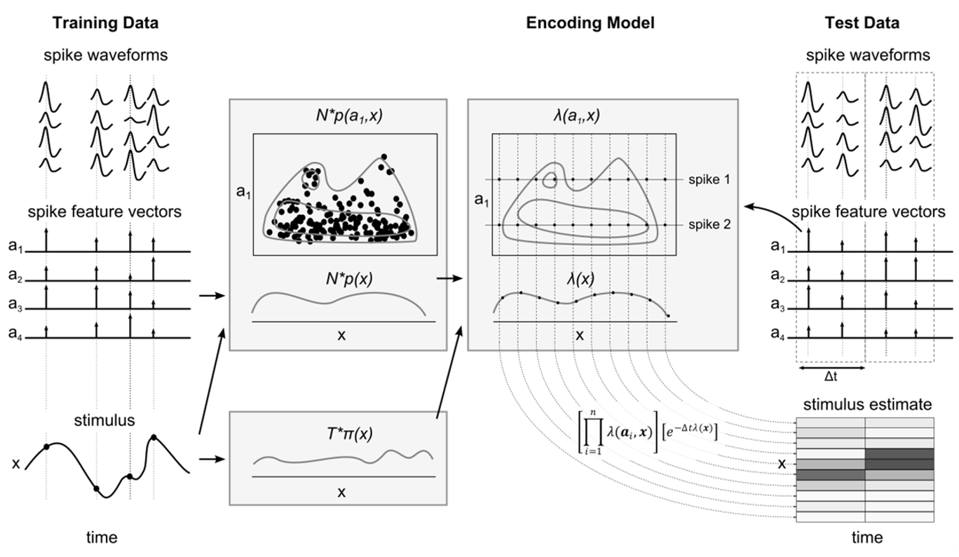
The likelhood for a single spike data source is fully determined by a rate function, \(\lambda_k \left(\boldsymbol{a},\boldsymbol{x}\right)\), that expresses the mean rate of spikes with certain waveform features for stimulus \(\boldsymbol{x}\).

As we have seen in the section on tuning curves, rate functions can be computed as the ratio between spike count probability and a stimulus occupancy probability:

\[\lambda(\boldsymbol{a},\boldsymbol{x})=\frac{N}{T}\frac{p_{spike}(\boldsymbol{a},\boldsymbol{x})}{p_{stimulus}(\boldsymbol{x})}\]

Similarly, for the marginal rate function \(\lambda(\boldsymbol{x})\):

\[\lambda(\boldsymbol{x})=\frac{N}{T}\frac{p_{spike}(\boldsymbol{x})}{p_{stimulus}(\boldsymbol{x})}\]

We can now use cKDE to compute the rate functions and subsequently calculate the likelihoods for neural decoding.

Python API neural decoding

Functions for cKDE-based neural decoding are part of the fklab-compressed-decoder package and available under the compressed_kde.decode module.

Apart from the space, grid and mixture objects described above, the API includes classes for the stimulus occupancy (Stimulus), Poisson likelihoods (PoissonLikelihood) and decoder (Decoder).

Stimulus

The Stimulus class represents the stimulus occupancy distribution \(p_{stimulus}(\boldsymbol{x})\). To construct a Stimulus object, provide a stimulus space and a grid of points for evaluation of the density. In addition, indicate the duration of a single stimulus (it is assumed that all stimulus samples have equal duration) and the desired compression level.

stimulus = Stimulus(
    stimulus_space,          # Space object
    grid,                    # Grid object
    stimulus_duration = 1.,  # duration of single stimulus sample
    compression = 1.         # compression level
)

To add stimulus samples to the Stimulus object use the add_stimuli method. To add the same stimulus samples more than once, set the repetitions argument to a value other than 1.

stimulus.add_stimuli(
    stimuli,       # (nsamples,ndim) array with stimulus values
    repetitions=1  # number of times each stimulus sample should be added
)

Poisson likelihood

The PoissonLikelihood class represent the single data source likelihood \(P\left(\boldsymbol{A}_k|\boldsymbol{x}\right)\). To construct a likelihood object, provide a Space object that describes the spike features and a Stimulus object.

likelihood = PoissonLikelihood(
    spike_feature_space,  # space object
    stimulus              # stimulus object
)

In case no spike features are used for decoding, only the Stimulus object needs to be provided:

likelihood = PoissonLikelihood(
    stimulus              # stimulus object
)

To add spike events to the likelihood, use the add_events method. The spike data should be a 2D array with spikes as rows and spike features and stimulus values (in this order) concatenated along the columns. To add the same spike events multiple times, set the repetitions argument to a value other than 1.

likelihood.add_events(
    spike_features_and_stimulus, #(nspikes,nfeatures+ndim) array
    repetitions=1
)

Decoder

The Decoder class is a container for likelihood objects and performs decoding given new spike events and their features. To construct a decoder, pass a list of likelihood objects (one for each data source) that all share the same stimulus space. Optionally, provide an array with prior probabilities for all the grid points in the stimulus space.

decoder = Decoder(
    [likelihood,...],  # list of likelihood objects
    prior = []         # vector of prior probabilities
)

To compute the posterior probability for a single time window, use the decode method. Provide a list of spike feature arrays (one for each data source) and indicate the duration of the time window.

posterior = decoder.decode(
    [spike_features, ...],   # List of (nspike, nfeatures) spike features arrays
    delta                    # time window size
)

Sometimes, one may want to decode across multiple distinct stimulus space. For example, when simultaneously decoding position across multiple mazes. For these case, construct a decoder by passing a nested list of likelihoods, where the outer list represents the data sources (e.g., individual tetrodes) and the inner lists represent multiple stimulus spaces one would like to decode over. Optionally, provide prior probabilities for each stimulus space as a list of arrays.

decoder = Decoder(
    [[likelihood,...],[likelihood,...],...],  # nested list of likelihoods
    priors = []                               # list of priors
)

To compute the posterior probability, use the decode method as before, with a list of spike feature arrays. To compute the posterior only for one of the stimulus space, use the decode_single method with zero-based index of the stimulus space:

posterior = decoder.decode_single(
    [spike_features, ...],   # List of (nspike, nfeatures) spike features arrays
    delta,                   # time window size
    index                    # index of stimulus space
)

Cross-validation

To characterize the performance of a decoder, one should use different data for training the model (i.e. the data used to build the likelihoods) and for testing the model (i.e. the data used for computing the posterior). Using the same data for training and testing a model leads to overfitting and poor generalization to future data samples. For more information cross-validation, see here.

The solution is to split the data into separate training and test data sets. Note that if (hyper) parameters need to be optimized, then you need to use nested cross validation (i.e., split the training data set in two parts - one part for training the model with a certain (hyper)parameter value and the other part for evaluating the model performance).

There are multiple ways of splitting the data into traing and test data sets. To make optimal use of the data, one can make multiple training/test data splits and average the results.

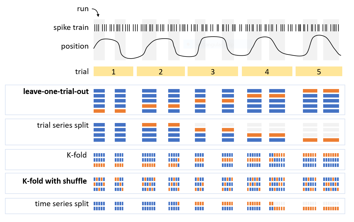
The figure below illustrates a few ways of splitting data. If the experiment naturally contains trials, then a leave-one-trial-out approach can be used in which one trial is selected for testing and all other trials are used for training the decoder. This is repeated until all trials have been used for testing exactly once.

Another common approach is K-fold cross-validation in which \(\frac{100\%}{K}\) of the time windows for decoding is selected for testing and the remaining time windows are used for training. Shuffling of the time windows could be benificial if there are systematic changes over time that hurt decoding performance.

Evaluation of decoding performance

To evaluate the performance of a decoder, you compare the decoded stimulus value \(\hat{\boldsymbol{x}}\) to the real stimulus value \(\boldsymbol{x}\). First, determine the posterior mode \(\underset{\boldsymbol{x}}{\mathrm{argmax}}(posterior\left(\boldsymbol{x}\right))\) as the stimulus value with highest posterior probability. Next, compute the distance between the decoded and real stimulus value, which is the decoding error. Because the distance computation depends on the stimulus space (e.g., the norm for euclidean space, circular difference for circular space, etc.), it is advisable to use the distance method of a space object, which will compute the pair-wise distance between stimulus values separately for each stimulus dimension:

distance = space.distance(
    x,  # (ndim,) or (n,ndim) array
    y   # (ndim,) or (n,ndim) array
)

For a multivariate stimulus space, there are two options to determine the posterior mode: either on the full multi-dimensional posterior or separately for each dimension after computing the marginal posterior distribution for that dimension (i.e., sum over all other dimensions).

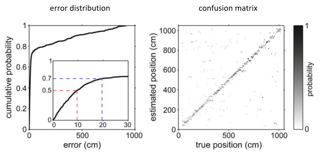
Once the decoding errors for all test data has been computed, you can visualize the (cumulative) error distribution and summarize the distribution (e.g. median error). See the example in the figure below (left). Note that for categorical stimulus variables, you would compute the percentage of correct estimates.

To further analyze the decoding performance, a confusion matrix can be constructed (see example on the right in figure below). The confusion matrix shows decoding performance for each stimulus value. A good decoder will have high values along the diagonal of the confusion matrix.

Workflow for neural decoding

Step 1: Gather your data

For all spikes, compute their features and determine the stimulus at the time of the spikes. Select time windows for encoding and decoding. For example, for decoding location in a maze, you could focus on times when the subject is actively moving. For hippocampal replay decoding, encoding would be performed with run data and decoding during activity bursts when subjects are sleeping or sitting quietly on track.

Step 2: Build stimulus occupancy object

Define the stimulus space and grid for evaluation of the probability densities (see here how to construct spaces and grids). Then, construct a Stimulus object and add stimulus samples.

Step 3: Build likelihoods

First, define the spike feature space. Next, for each spike data source construct a PoissonLikelihood object and add spike events with their features and stimulus value at the time of the spikes.

Step 4: Build decoder

Construct a Decoder object with all likelihoods.

Step 5: Decode

Compute the posterior distribution for each time bin with measured spike features.

Step 6: Cross-validation

Perform cross-validation and evaluate the decoding performance.